Summer 2026 Reflections: MathPath
I spent two weeks of July at MathPath, a four-week math summer program for 11-14 year olds. At camp, students took two breakouts each week, with morning breakouts meeting for 65 min per day across 5 days and evening breakouts meeting for 80 min per day across 4 days. Each breakout also had 25 minutes of daily conferencing time for homework, except for the last day of the breakout.
The four topics courses I taught were Graph Coloring, Amazing Algorithmic Race, Climate & Chaos, and Conditional Probability & Bayes’ Theorem. Algorithms and Climate & Chaos drew on breakouts of the same names that I had taught at MathPath 2022, as well as my recent teaching of Algorithms and Dynamical Systems at Camp Conway. Graph Coloring is a frequently taught MathPath course, so I had some others’ materials to look at there. Conditional Probability & Bayes’ Theorem was new.
Graph Coloring
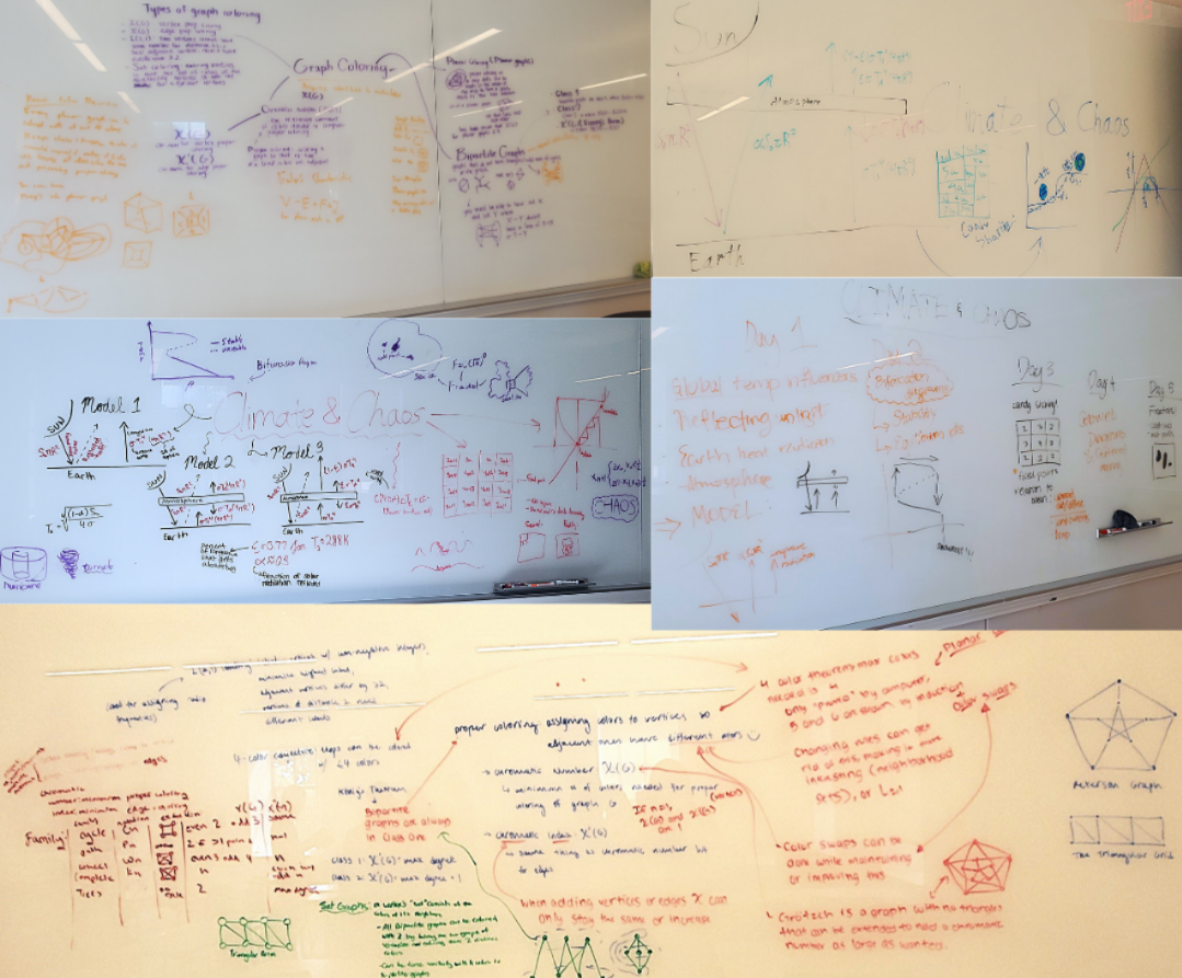
I saw the Five Color Theorem as the mid-week highlight of this course, but part of my goal was showing how many different ways we can think about graph coloring or labeling. So my goal here was breadth over depth, with lots of exploration. I was also trying to build up some patterns when looking at those new types of coloring/labeling: looking at families of graphs, looking for bounds in terms of other features of the graph. Here’s what the week looked like:
Day 1: What are proper vertex colorings, and what is chromatic number? What are proper edge colorings, and what is chromatic index? What do these look like for common families of graphs? Can we come up with any useful bounds?
Day 2: Proof of the chromatic index of trees to follow up on some student conjectures from previous day and to introduce induction for graphs, intro to planar graphs and Four Color Conjecture, student examples to show at least four colors are needed
Day 3: Proofs of Six Color Theorem and Five Color Theorem, discussion of Four Color Theorem
Day 4: Explorations of \(L(2,1)\) labelings and set colorings
Day 5: Explorations of game-chromatic number, wrap-up
I adapted some MathPath 2022 materials from Emily Olson for structuring the proof of the Six Color Theorem and for introducing Kempe chains. I had thought about doing a Parsons problem for the Six Color Theorem instead, but having a proof outline worked out better logistically and I think pointed more in the direction of writing out their reasoning. The warmup of a similar proof outline and structure for the chromatic index of trees the day before helped a lot. And really working with the Kempe chain idea before seeing it in the Five Color Theorem was also helpful!
I left the explorations of other types of colorings/labelings quite open on Days 4 and 5, though I did prompt pretty heavily in the direction of looking at families of graphs. On Day 4, we spent most of class on \(L(2,1)\) labelings and so didn’t have as much time on set colorings as would have been nice, given that they’re a bit different from the other types we looked at. But just \(L(2,1)\) labelings for the breakout would have required point students in a structured way in more directions, I think.
Homework/conferencing time problems throughout the week had a lot of different flavors: coloring/labeling some particular graphs, applied/modeling problems, small proofs of more results, writing up explorations and questions. I also used these problems to sneak in a couple more variations: balanced colorings, uniquely colorable, list coloring. In the future I would want to encourage folks more in the writing direction vs just finding labelings. By the end of the week, I was phrasing problems to require some writing about how they knew they couldn’t do better than the labeling they’d found.
The main thing I want to think about more with this breakout is how to structure the explorations of new types of coloring/labeling well. What kinds of questions and suggestions leave lots of room for students to figure things out and conjecture while nudging them towards useful families or questions?
Algorithms
My plan for this breakout was to focus on time complexity, sorting lists, and finding paths in graphs. Here’s the rough outline of where things went:
Day 1: What is an algorithm, and what makes a good one? Did an exercise of writing instructions for others to draw a simple picture, played around with some arithmetic algorithms, and designed algorithms to find the minimum of a list.
Day 2: Time complexity. They looked at a visual pattern to describe how it grew and came up with patterns that grew slower or faster. From here, I introduced Big O notation. Sorting lists. I asked them to come up with an algorithm to sort an unsorted list and then to figure out its time complexity. We talked through the time complexity of mergesort in detail.
Day 3: Graph traversal. We looked at unweighted, undirected graphs, and I started by asking them to write an algorithm to find some path from a source vertex to each of the other vertices (if possible). After both breadth-frist search and depth-first search emerged, we talked about which one would work to find a shortest path. I gave them some time to try to adjust those algorithms to work for weighted edges, and then we talked through Dijkstra’s algorithm
Day 4: Algorithmic puzzles and games. They spent most of the time working on a solitaire version of toads & frogs and Julia Robinson Mathematics Festival’s apple picking game, particularly the 2D version. Then we did some wrap-up.
Popular conferencing time/homework problems along the way included algorithms for river crossing, flipping pancakes, reorganizing checkers, and finding connected components in a graph.
Integrating puzzles throughout the week became part of my plan after feeling like it would have helped the pace and feeling of my Camp Conway Algorithms course, and that worked really well here! I do wish I’d started class on Wednesday through Friday by having students present some solutions from the previous day’s homework; I think that would have gotten us talking about more algorithms in a useful way.
A couple of things here that I’d like to work on or think about more:
Sorting is nice as a case where it’s not too hard to find best and worst cases to talk about time complexity for different algorithms, and students often come up with multiple algorithms that work. But it’s also the spot in the material where prior experience most strongly varies (and perhaps is also an “oh, I’ve seen that before” moment that keeps students from taking the course/breakout, though I’m less sure of that). What other directions of algorithms could I extend in, and is there something else that can take the spot of sorting for being a good intro playground for time complexity?
“Complete, Correct, and Finite” is an important idea about what algorithms should look like, but it’s not a very satisfying theme. What’s a more satisfying idea that I want to keep coming back to in this breakout?
Climate & Chaos
My 2022 notes on this breakout indicate that it basically had two sections: energy balance models and 1D discrete maps leading to chaos, with a connection to the Lorenz 63 equations at the end. MathPath faculty colleague Dr. Nick had taught two weeks of breakouts on dynamical systems, and I had a pretty vocal overlap of campers with those breakouts, so I wanted less of this to be an intro to 1D discrete maps than when I had last taught it. At the same time, I had lots of students who hadn’t taken any dynamical systems, so I didn’t want to skip over those ideas. Here’s where I ended up:
Day 1: What influences global temperature? Then we built two energy balance models, one without an atmosphere and one with an atmosphere that absorbs all the surface longwave.
Day 2: Making the energy balance models more sophisticated, either with a parameter for how much longwave is absorbed and emitted by the atmosphere or with a temperature-dependent albedo. The latter led to multiple equilibria and a discussion of stability, bifurcations, and snowball Earth.
Day 3: Exploring a dynamical system on a grid, inspired by candy sharing and chip-firing games. We started with a 2x2 or 3x3 grid of people, each with a given amount of candy. At each timestep, every person gives each of their neighbors (those who share a side in the grid) as many whole pieces of candy as possible, giving each neighbor the same amount of candy. What happens to the amount of candy each person has over time? Students looked for fixed points and periodic orbits, and then we came up with some ways that changing rules of this game might help us to think about models of ocean dynamics.
Day 4: 1D discrete maps. We looked at some non-chaotic maps first to introduce what fixed points and periodic orbits look like here and how to use cobweb diagrams. Then I gave students the tent map to play with. After a while, we defined chaos and related the tent map’s behavior to the weather’s chaotic behavior.
Day 5: Fractal dimension, sea ice melt ponds, and clouds. Also some wrap-up and brief diversions at the beginning into aerosols and tornadoes vs hurricanes!
In the future, I’d like to do a better job of closing the lesson on Days 3 and 4 with better explanations of how these simple models are and aren’t related to models that people actually use of what happens in the ocean and atmosphere. On Day 4, I didn’t end up showing anything directly related to Lorenz; I thought I could get away with an advection vs dispersion handwave, and I absolutely Could Not. (Some combination of not being prepared enough for the handwave and, in my undergrad advisor’s words, the students not “knowing in [their] gut what it means to build patterns from modes.”) An explanation that actually looked at the Lorenz attractor and pulled out the pattern of highest \(z\) values, relating that to energy and to (almost) the shape of the tent map, might land better, though it’s a lot of steps to take.
Day 5 also needs some work. Ideally, this would be an activity that would introduce fractals (not just self-similar shapes) and then look at dimension, probably box-counting and then area-perimeter ways of thinking about dimension. After that, we could look at the papers I linked in the Day 5 description.
Homework is a little tricky for this breakout sometimes. There are problems that are good fits but need some intro to a different context or some nudges in a modeling direction, and it went better to explain those orally than in writing. These are problems about things like nighttime cooling, atmospheric stability (related to lapse rate), and bifurcations in Stommel’s two box ocean model.
A student asked a question on Day 1 about energy balance on other planets that would have been a perfect homework problem, so I included models for Mercury, Venus, and Mars on a later homework! I plan to move that forward to Day 1 for the future; it’s much more accessible than the problems I actually gave on Day 1, and it’s a great question.
Conditional Probability & Bayes’ Theorem
This breakout was brand new! I drew on materials I’ve used in Stat Analysis and ProbStat II for introducing Bayesian stats (including some POGIL materials, lots of problems and approaches from Bayes Rules!, and some problems and the table approach from Think Bayes). Here’s the outline of the week:
Day 1: Building up ideas about conditional probability and total probability. We got to Bayes’ right at the end.
Day 2: Bayes’ Theorem! Using it directly, using a table as an organizer for seeing what’s going on, lots of different problems and applications.
Day 3: More Bayes’ applications, intro to binomial distribution and beta distribution, Beta-Binomial models
Day 4: Bayes’ problem carnival
This breakout lost steam later in the week. Some of that was it being the afternoon of Week 4 and all of us being a little tired and less focused. But I think Days 3 and 4 would have gone better with a stronger intro to the beta distributions and the kinds of problems where we want it as our prior. Here’s what I think would have worked better:
An example and a problem or two with binomial data but discrete hypotheses (I thought about this and then didn’t do it for some reason…);
Drawing probability mass functions for our priors and posteriors in the discrete hypothesis case as a bridge to probability distribution functions;
Discussion of that transition from discrete to continuous before showing the beta distribution, maybe having them sketch some priors for different scenarios;
THEN introducing the beta distribution and patterns in how it depends on its parameters;
Better addressing of the idea of “conjugate prior.”
That would likely have taken up more time on Day 3 but more effectively, maybe spreading into Day 4, and then we would have had Beta-Binomial problems and wrap-up to focus on for Day 4.
(There is definitely a pattern between this breakout and Climate & Chaos of trying to do things that are calculus without doing calculus.)
On Day 3 homework, I tried to have students write their own Bayes’ problems. The more closely they imitated a problem I’d given them, the more successful they were. It’s tricky to figure out the right combination of given and missing information to write a successful problem here. But I think spending some time trying to see those patterns and thinking about what we can figure out what from what information could be worthwhile.
One last thing I want to change for the future: the title of this breakout. This title is long and a little dry. I’m also wondering if I should say something in the description and Show & Tell in the contest problem direction, but I’m conflicted about it.
Overall
I told someone that MathPath is kind of a firehose (complimentary), with all the different math that students are seeing over the course of four weeks, in contrast to some other enrichment experiences that are more in depth on fewer ideas. The context-switching can be a lot as faculty, too, but it was exciting to get to teach so many different parts of what I’ve done in the mathematical sciences!